Transfer Learning on Habana Gaudi for Object Detection with Transportation Dataset
Key Points
- Transfer Learning is an efficient way to train an existing model on a new and unique set of data, taking advantage a model’s existing capability and weights to work on the new dataset with equivalent accuracy and significantly less training time.
- This paper will show the steps to start with the EfficientDet model from Habana Model-References that was originally trained on the COCO dataset in 2.7 days on 8 Gaudi HPUs, and fine-tuning the model on a smaller Road Sign Detection dataset in just 30 minutes. To run this fine-tuning on the AWS DL1 Instance would result in a savings of ~$850 dollars compared to a full model training.
Transfer learning is a common approach in AI where knowledge learned on one dataset or task can be applied to a new target dataset or task. It leverages generalizable knowledge learned from a source task to a target task. The knowledge learned from the source task is stored in the trained weights, which can be directly applied to the target domain. Therefore, the target task can be addressed with better performance. The pre-trained model serves as an initial point for training for the target domain. From the optimization point of view, good initial weights can make the model closer to the optimal solution, which in turn can converge the training faster.
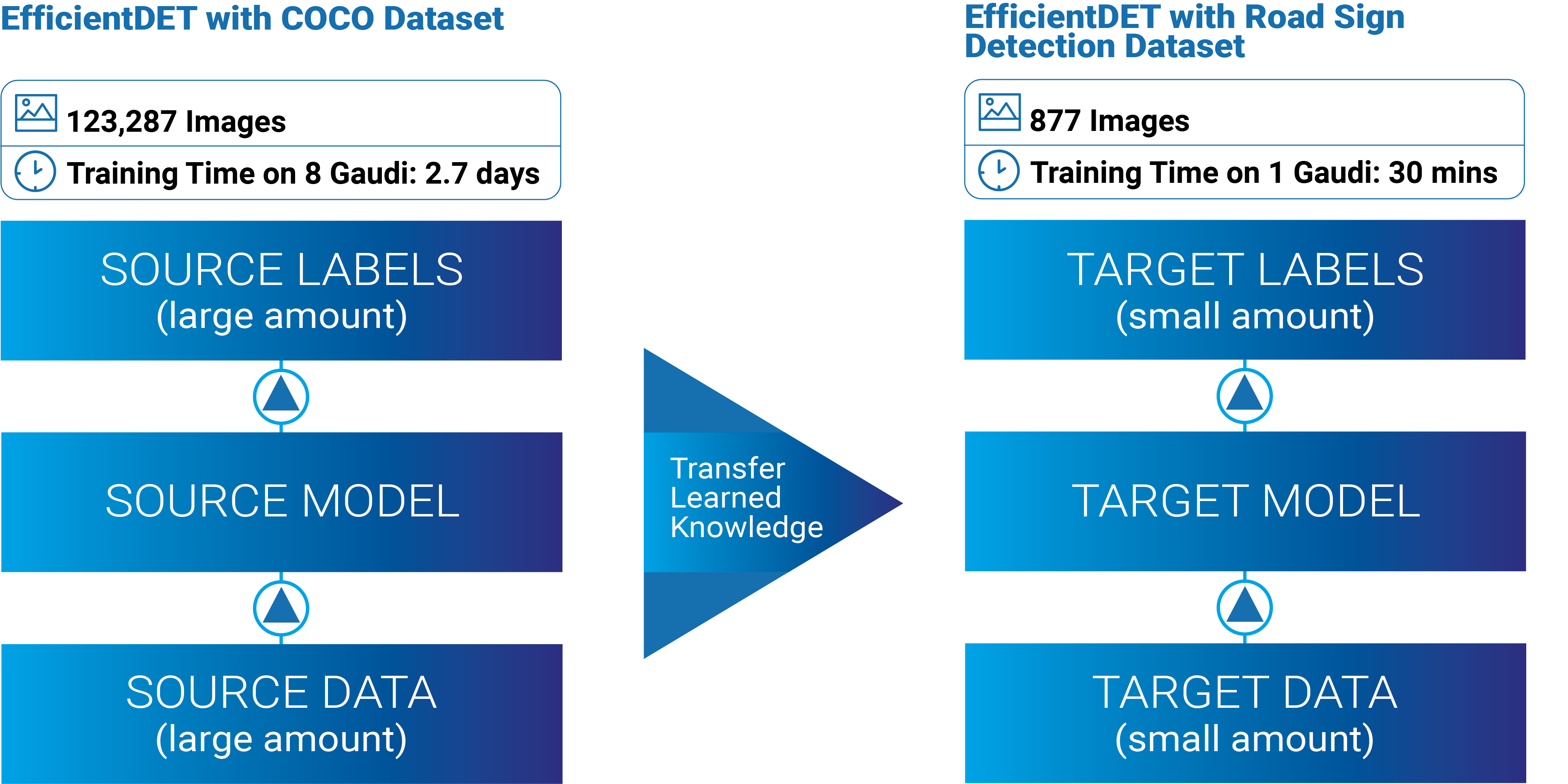
Considering that it takes days or even weeks to train a complex deep learning model from scratch, transfer learning is a more efficient approach. Transfer learning can also prevent overfitting, especially when the dataset size in the target domain is not large enough to train a deep neural network from scratch.
In this specific case, we are showing how a set of checkpoints fully trained on Gaudi are used for this Transfer Learning example. In general, the saved pretrained model can be used on different architectures. For example, you can pretrain a model using Habana Gaudi AI Processor, save it, and later fine tune the model using a CPU. Or you can load a publicly available pretrained model, originally pretrained on GPU, and continue training or fine tuning it on Habana Gaudi AI processor.
Habana provides a GitHub Model-References repository with both TensorFlow and PyTorch Deep Learning models optimized on Habana Gaudi, covering computer vision, natural language processing, audio, and recommendation systems. Additionally, Habana provides pre-trained checkpoints in the Habana Catalog for various models. The training scripts as well as checkpoints allow users to easily perform transfer learning tasks on Habana devices.
In this post, we describe how to apply transfer learning to TensorFlow EfficientDet-D0 on Habana Gaudi. It proves that transfer learning with only a few epochs can train a model to detect objects in a new dataset using the knowledge learned from the dataset used for pre-training.
The pre-trained EfficientDet-D0 model that Habana provides was trained on Habana Gaudi with MS COCO dataset using TensorFlow. The target dataset used in this example is road sign detection dataset. It is an open-source dataset with traffic sign images and annotations for detection tasks. The dataset can be downloaded from Kaggle datasets then preprocessed using the ‘create_roadsign_tfrecord.py’ located in Habana’s Gaudi-tutorial repository. The preprocess script reads an image and annotation information, then converts them into TFRecord format.
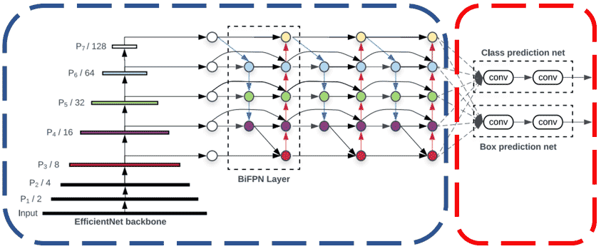
Transfer learning with EfficientDet-D0 trains the last few prediction layers of the model on a target dataset while freezing the base networks. In Figure 2 EfficientDet Architecturewhich represents the architecture of EfficientDet, the portions enclosed with the blue box are frozen while the prediction networks enclosed with the red box are being trained. Except for the prediction networks, the remaining layers such as EfficientNet backbone and FPN weights are frozen so that general features learned during pre-training are not disturbed. The prediction networks of the pre-trained model are replaced for the new dataset and randomly initialized. Then the new prediction networks are trained on the road sign detection dataset from scratch.
The EfficientDet-D0 model was trained for ten epochs for transfer learning with batch size 2. After hyperparameter tuning, the set of hyperparameters in Table 1 are identified to be useful for convergence of the model. The hyperparameters for the model training is included in ‘hparams_config_tl.py’ in the repository, so users can easily tune them by passing them in the run command. The hyperparameters used in each step are discussed in the following.
| use_bfloat16 | True |
| num_classes | 5 |
| var_freeze_expr | ‘(efficientnet|fpn_cells|resample_p6)’ |
| train_scale_min | 0.8 |
| train_scale_max | 1.2 |
| lr_warmup_epoch | 0 |
| learning_rate | 0.08 |
- Habana mixed precision training is enabled by ‘use_bfloat16’. It is recommended to enable mixed precision training to improve training performance and reducing memory usage of Gaudi.
- ‘num_classes’ and ‘var_freeze_expr’ are used to modify the model structure for feature extraction. ‘num_classes’ is the number of object categories in the dataset. The road sign detection dataset has 5 classes, background, traffic light, stop, speed limit, and crosswalk. When replacing the class prediction networks for feature extraction, its size is determined by ‘num_classes’. To specify layers to freeze, a regular expression of layers is passed to ‘var_freeze_expr’. “(efficientnet|fpn_cells|resample_p6)” is set so that backbone and FPN weights are excluded from training and only prediction networks are trained.
- ‘train_scale_min’ and ‘train_scale_max’ are for scale jittering. Each input image is resized with a randomly sampled scale factor between ‘train_scale_min’ and ‘train_scale_max’ (Simonyan & Zisserman, 2015). This can increase the diversity of the training dataset, making the model more robust.
- The learning rate can be set using ‘learning_rate’ and ‘lr_warmup_epoch’. ‘learning_rate’ was set to 0.08. This learning rate is adjusted before training in proportion to the ratio of the batch size to the default batch size of 64. Thus, the actual learning rate values are 0.0025. Learning rate warm-up was skipped by setting ‘lr_warmup_epoch’ to 0.
With the transfer learning process described above, the model is trained with 789 training images and evaluated with 88 validation images. The training is performed using SynapseAI version 1.7 with TensorFlow 2.9.1 on a single Habana Gaudi. The entire transfer learning process takes approximately 30 minutes, and the model achieved the validation accuracy AP @IoU=0.5:0.95 of 0.328. Table 2 shows the evaluation results after training. Please note that Average Precision and Average Recall values marked as -1.000 in Table 2 mean the corresponding area categories (medium and large) are absent in the validation dataset. The area category depends on the pixel area of an object in images (COCOdataset, 2022).
| AP Measurement | Value |
|---|---|
| Average Precision (AP) @[ IoU=0.50:0.95 | area= all | maxDets=100 ] | 0.328 |
| Average Precision (AP) @[ IoU=0.50 | area= all | maxDets=100 ] | 0.467 |
| Average Precision (AP) @[ IoU=0.75 | area= all | maxDets=100 ] | 0.377 |
| Average Precision (AP) @[ IoU=0.50:0.95 | area= small | maxDets=100 ] | 0.565 |
| Average Precision (AP) @[ IoU=0.50:0.95 | area=medium | maxDets=100 ] | -1.000 |
| Average Precision (AP) @[ IoU=0.50:0.95 | area= large | maxDets=100 ] | -1.000 |
| Average Recall (AR) @[ IoU=0.50:0.95 | area= all | maxDets= 1 ] | 0.494 |
| Average Recall (AR) @[ IoU=0.50:0.95 | area= all | maxDets= 10 ] | 0.633 |
| Average Recall (AR) @[ IoU=0.50:0.95 | area= all | maxDets=100 ] | 0.647 |
| Average Recall (AR) @[ IoU=0.50:0.95 | area= small | maxDets=100 ] | 0.647 |
| Average Recall (AR) @[ IoU=0.50:0.95 | area=medium | maxDets=100 ] | -1.000 |
| Average Recall (AR) @[ IoU=0.50:0.95 | area= large | maxDets=100 ] | -1.000 |
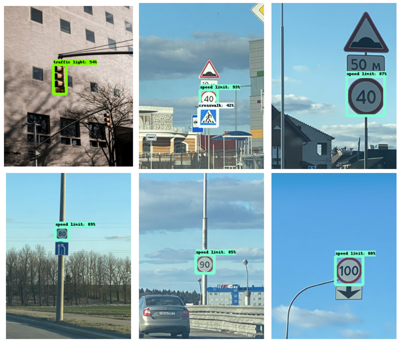
In addition to evaluation, inference was performed using the model generated from the transfer learning process with sample images below. The inference results are visualized in Figure 2 Inference results, which presents input images with bounding boxes and prediction probabilities from the model.
In conclusion, from the example in this post we can learn how to apply transfer learning technique to the pre-trained model on Habana Gaudi on a custom dataset. With the help of training scripts in the Model-References repository as well as the pre-trained model provided by Habana, users can perform training of a deep learning neural network on a custom dataset and achieve considerable accuracy with better performance and cost efficiency. You can refer to our code example in our Tutorial to reproduce these results.
References
Li, J. (2020, November 3). ML6 blog. Retrieved from Retraining EfficientDet for High-Accuracy Object Detection: https://blog.ml6.eu/retraining-efficientdet-for-high-accuracy-object-detection-961e906cae8
Simonyan, K., & Zisserman, A. (2015). Very Deep Convolutional Networks for Large-Scale Image Recognition. ICLR.
TensorFlow. (2022). TensorFlow Guide. Retrieved from https://www.tensorflow.org/guide/keras/transfer_learning#fine-tuning
