An adaptation of Intro to Autoencoders tutorial using Habana Gaudi AI processors.
This tutorial introduces autoencoders with three examples: the basics, image denoising, and anomaly detection.
An autoencoder is a special type of neural network that is trained to copy its input to its output. For example, given an image of a handwritten digit, an autoencoder first encodes the image into a lower dimensional latent representation, then decodes the latent representation back to an image. An autoencoder learns to compress the data while minimizing the reconstruction error.
To learn more about autoencoders, please consider reading chapter 14 from Deep Learning by Ian Goodfellow, Yoshua Bengio, and Aaron Courville.
Import TensorFlow and other libraries
import matplotlib.pyplot as plt
import numpy as np
import pandas as pd
import tensorflow as tf

from sklearn.metrics import accuracy_score, precision_score, recall_score
from sklearn.model_selection import train_test_split
from tensorflow.keras import layers, losses
from tensorflow.keras.datasets import fashion_mnist
from tensorflow.keras.models import Model
Import and enable Habana TensorFlow module
Let’s enable a single Gaudi device by loading the Habana module:
import habana_frameworks.tensorflow as htf
htf.load_habana_module()
Load the dataset
To start, you will train the basic autoencoder using the Fashon MNIST dataset. Each image in this dataset is 28×28 pixels.
(x_train, _), (x_test, _) = fashion_mnist.load_data()

x_train = x_train.astype('float32') / 255.
x_test = x_test.astype('float32') / 255.

print (x_train.shape)
print (x_test.shape)
(60000, 28, 28)
(10000, 28, 28)First example: Basic autoencoder
Define an autoencoder with two Dense layers: an encoder, which compresses the images into a 64 dimensional latent vector, and a decoder, that reconstructs the original image from the latent space.
To define your model, use the Keras Model Subclassing API.
latent_dim = 64

class Autoencoder(Model):
  def __init__(self, latent_dim):
    super(Autoencoder, self).__init__()
    self.latent_dim = latent_dim
    self.encoder = tf.keras.Sequential([
      layers.Flatten(),
      layers.Dense(latent_dim, activation='relu'),
    ])
    self.decoder = tf.keras.Sequential([
      layers.Dense(784, activation='sigmoid'),
      layers.Reshape((28, 28))
    ])

  def call(self, x):
    encoded = self.encoder(x)
    decoded = self.decoder(encoded)
    return decoded

autoencoder = Autoencoder(latent_dim)
autoencoder.compile(optimizer='adam', loss=losses.MeanSquaredError())Train the model using x_train as both the input and the target. The encoder will learn to compress the dataset from 784 dimensions to the latent space, and the decoder will learn to reconstruct the original images. .
autoencoder.fit(x_train, x_train,
                epochs=10,
                shuffle=True,
                validation_batch_size=40,
                validation_data=(x_test, x_test))
Epoch 1/10
1875/1875 [==============================] - 9s 3ms/step - loss: 0.0241 - val_loss: 0.0132
Epoch 2/10
1875/1875 [==============================] - 6s 3ms/step - loss: 0.0116 - val_loss: 0.0105
Epoch 3/10
1875/1875 [==============================] - 6s 3ms/step - loss: 0.0100 - val_loss: 0.0097
Epoch 4/10
1875/1875 [==============================] - 6s 3ms/step - loss: 0.0094 - val_loss: 0.0093
Epoch 5/10
1875/1875 [==============================] - 6s 3ms/step - loss: 0.0092 - val_loss: 0.0093
Epoch 6/10
1875/1875 [==============================] - 6s 3ms/step - loss: 0.0090 - val_loss: 0.0091
Epoch 7/10
1875/1875 [==============================] - 6s 3ms/step - loss: 0.0089 - val_loss: 0.0089
Epoch 8/10
1875/1875 [==============================] - 6s 3ms/step - loss: 0.0089 - val_loss: 0.0089
Epoch 9/10
1875/1875 [==============================] - 6s 3ms/step - loss: 0.0088 - val_loss: 0.0089
Epoch 10/10
1875/1875 [==============================] - 6s 3ms/step - loss: 0.0087 - val_loss: 0.0089
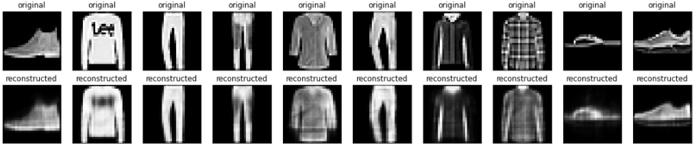
<keras.callbacks.History at 0x7f8e7cd97450>Code language: HTML, XML (xml)Now that the model is trained, let’s test it by encoding and decoding images from the test set.
encoded_imgs = autoencoder.encoder(x_test).numpy()
decoded_imgs = autoencoder.decoder(encoded_imgs).numpy()
n = 10
plt.figure(figsize=(20, 4))
for i in range(n):
# display original
ax = plt.subplot(2, n, i + 1)
plt.imshow(x_test[i])
plt.title("original")
plt.gray()
ax.get_xaxis().set_visible(False)
ax.get_yaxis().set_visible(False)
# display reconstruction
ax = plt.subplot(2, n, i + 1 + n)
plt.imshow(decoded_imgs[i])
plt.title("reconstructed")
plt.gray()
ax.get_xaxis().set_visible(False)
ax.get_yaxis().set_visible(False)
plt.show()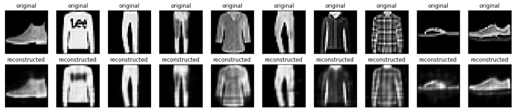
Second example: Image denoising
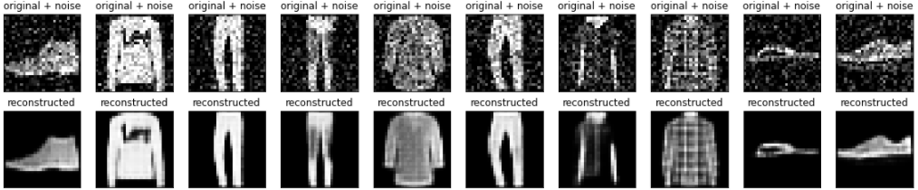
An autoencoder can also be trained to remove noise from images. In the following section, you will create a noisy version of the Fashion MNIST dataset by applying random noise to each image. You will then train an autoencoder using the noisy image as input, and the original image as the target.
Let’s reimport the dataset to omit the modifications made earlier.
(x_train, _), (x_test, _) = fashion_mnist.load_data()x_train = x_train.astype('float32') / 255.
x_test = x_test.astype('float32') / 255.
x_train = x_train[..., tf.newaxis]
x_test = x_test[..., tf.newaxis]
print(x_train.shape)(60000, 28, 28, 1)Adding random noise to the images
noise_factor = 0.2
x_train_noisy = x_train + noise_factor * tf.random.normal(shape=x_train.shape)
x_test_noisy = x_test + noise_factor * tf.random.normal(shape=x_test.shape)

x_train_noisy = tf.clip_by_value(x_train_noisy, clip_value_min=0., clip_value_max=1.)
x_test_noisy = tf.clip_by_value(x_test_noisy, clip_value_min=0., clip_value_max=1.)
Plot the noisy images.
n = 10
plt.figure(figsize=(20, 2))
for i in range(n):
    ax = plt.subplot(1, n, i + 1)
    plt.title("original + noise")
    plt.imshow(tf.squeeze(x_test_noisy[i]))
    plt.gray()
plt.show()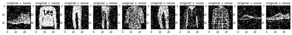
Define a convolutional autoencoder
In this example, you will train a convolutional autoencoder using Conv2D layers in the encoder, and Conv2DTranspose layers in the decoder.
class Denoise(Model):
  def __init__(self):
    super(Denoise, self).__init__()
    self.encoder = tf.keras.Sequential([
      layers.Input(shape=(28, 28, 1)),
      layers.Conv2D(16, (3, 3), activation='relu', padding='same', strides=2),
      layers.Conv2D(8, (3, 3), activation='relu', padding='same', strides=2)])

    self.decoder = tf.keras.Sequential([
      layers.Conv2DTranspose(8, kernel_size=3, strides=2, activation='relu', padding='same'),
      layers.Conv2DTranspose(16, kernel_size=3, strides=2, activation='relu', padding='same'),
      layers.Conv2D(1, kernel_size=(3, 3), activation='sigmoid', padding='same')])

  def call(self, x):
    encoded = self.encoder(x)
    decoded = self.decoder(encoded)
    return decoded

autoencoder = Denoise()
autoencoder.compile(optimizer='adam', loss=losses.MeanSquaredError())autoencoder.fit(x_train_noisy, x_train,
epochs=10,
shuffle=True,
batch_size=32,
validation_batch_size=40,
validation_data=(x_test_noisy, x_test))Epoch 1/10
1875/1875 [==============================] - 10s 4ms/step - loss: 0.0166 - val_loss: 0.0097
Epoch 2/10
1875/1875 [==============================] - 7s 3ms/step - loss: 0.0091 - val_loss: 0.0086
Epoch 3/10
1875/1875 [==============================] - 7s 4ms/step - loss: 0.0082 - val_loss: 0.0079
Epoch 4/10
1875/1875 [==============================] - 7s 4ms/step - loss: 0.0077 - val_loss: 0.0077
Epoch 5/10
1875/1875 [==============================] - 7s 4ms/step - loss: 0.0075 - val_loss: 0.0074
Epoch 6/10
1875/1875 [==============================] - 7s 3ms/step - loss: 0.0073 - val_loss: 0.0073
Epoch 7/10
1875/1875 [==============================] - 7s 4ms/step - loss: 0.0072 - val_loss: 0.0072
Epoch 8/10
1875/1875 [==============================] - 7s 4ms/step - loss: 0.0071 - val_loss: 0.0071
Epoch 9/10
1875/1875 [==============================] - 7s 3ms/step - loss: 0.0070 - val_loss: 0.0070
Epoch 10/10
1875/1875 [==============================] - 7s 4ms/step - loss: 0.0069 - val_loss: 0.0069
<keras.callbacks.History at 0x7f8d98a00b90>Code language: HTML, XML (xml)Let’s take a look at a summary of the encoder. Notice how the images are downsampled from 28×28 to 7×7.
autoencoder.encoder.summary()Model: "sequential_2"
_________________________________________________________________
Layer (type) Output Shape Param #
=================================================================
conv2d (Conv2D) (None, 14, 14, 16) 160
_________________________________________________________________
conv2d_1 (Conv2D) (None, 7, 7, 8) 1160
=================================================================
Total params: 1,320
Trainable params: 1,320
Non-trainable params: 0Code language: PHP (php)The decoder upsamples the images back from 7×7 to 28×28.
autoencoder.decoder.summary()Model: "sequential_3"
_________________________________________________________________
Layer (type) Output Shape Param #
=================================================================
conv2d_transpose (Conv2DTran (None, 14, 14, 8) 584
_________________________________________________________________
conv2d_transpose_1 (Conv2DTr (None, 28, 28, 16) 1168
_________________________________________________________________
conv2d_2 (Conv2D) (None, 28, 28, 1) 145
=================================================================
Total params: 1,897
Trainable params: 1,897
Non-trainable params: 0Code language: PHP (php)Plotting both the noisy images and the denoised images produced by the autoencoder.
encoded_imgs = autoencoder.encoder(x_test).numpy()
decoded_imgs = autoencoder.decoder(encoded_imgs).numpy()
n = 10
plt.figure(figsize=(20, 4))
for i in range(n):
# display original + noise
ax = plt.subplot(2, n, i + 1)
plt.title("original + noise")
plt.imshow(tf.squeeze(x_test_noisy[i]))
plt.gray()
ax.get_xaxis().set_visible(False)
ax.get_yaxis().set_visible(False)
# display reconstruction
bx = plt.subplot(2, n, i + n + 1)
plt.title("reconstructed")
plt.imshow(tf.squeeze(decoded_imgs[i]))
plt.gray()
bx.get_xaxis().set_visible(False)
bx.get_yaxis().set_visible(False)
plt.show()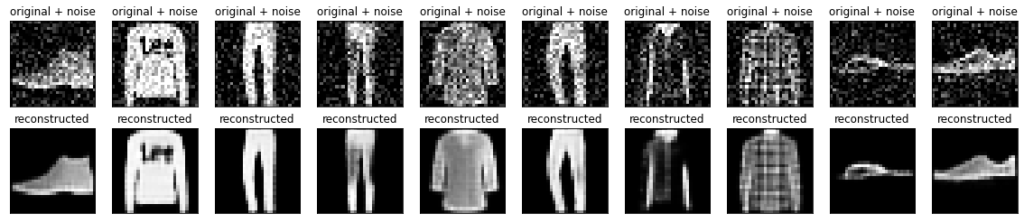
Third example: Anomaly detection
Overview
In this example, you will train an autoencoder to detect anomalies on the ECG5000 dataset. This dataset contains 5,000 Electrocardiograms, each with 140 data points. You will use a simplified version of the dataset, where each example has been labeled either 0 (corresponding to an abnormal rhythm), or 1 (corresponding to a normal rhythm). You are interested in identifying the abnormal rhythms.
Note: This is a labeled dataset, so you could phrase this as a supervised learning problem. The goal of this example is to illustrate anomaly detection concepts you can apply to larger datasets, where you do not have labels available (for example, if you had many thousands of normal rhythms, and only a small number of abnormal rhythms).
How will you detect anomalies using an autoencoder? Recall that an autoencoder is trained to minimize reconstruction error. You will train an autoencoder on the normal rhythms only, then use it to reconstruct all the data. Our hypothesis is that the abnormal rhythms will have higher reconstruction error. You will then classify a rhythm as an anomaly if the reconstruction error surpasses a fixed threshold.
Load ECG data
The dataset you will use is based on one from timeseriesclassification.com.
# Download the dataset
dataframe = pd.read_csv('http://storage.googleapis.com/download.tensorflow.org/data/ecg.csv', header=None)
raw_data = dataframe.values
dataframe.head()| 0 | 1 | 2 | 3 | 4 | 5 | 6 | 7 | 8 | 9 | … | 131 | 132 | 133 | 134 | 135 | 136 | 137 | 138 | 139 | 140 | |
|---|---|---|---|---|---|---|---|---|---|---|---|---|---|---|---|---|---|---|---|---|---|
| 0 | -0.112522 | -2.827204 | -3.773897 | -4.349751 | -4.376041 | -3.474986 | -2.181408 | -1.818286 | -1.250522 | -0.477492 | … | 0.792168 | 0.933541 | 0.796958 | 0.578621 | 0.257740 | 0.228077 | 0.123431 | 0.925286 | 0.193137 | 1.0 |
| 1 | -1.100878 | -3.996840 | -4.285843 | -4.506579 | -4.022377 | -3.234368 | -1.566126 | -0.992258 | -0.754680 | 0.042321 | … | 0.538356 | 0.656881 | 0.787490 | 0.724046 | 0.555784 | 0.476333 | 0.773820 | 1.119621 | -1.436250 | 1.0 |
| 2 | -0.567088 | -2.593450 | -3.874230 | -4.584095 | -4.187449 | -3.151462 | -1.742940 | -1.490659 | -1.183580 | -0.394229 | … | 0.886073 | 0.531452 | 0.311377 | -0.021919 | -0.713683 | -0.532197 | 0.321097 | 0.904227 | -0.421797 | 1.0 |
| 3 | 0.490473 | -1.914407 | -3.616364 | -4.318823 | -4.268016 | -3.881110 | -2.993280 | -1.671131 | -1.333884 | -0.965629 | … | 0.350816 | 0.499111 | 0.600345 | 0.842069 | 0.952074 | 0.990133 | 1.086798 | 1.403011 | -0.383564 | 1.0 |
| 4 | 0.800232 | -0.874252 | -2.384761 | -3.973292 | -4.338224 | -3.802422 | -2.534510 | -1.783423 | -1.594450 | -0.753199 | … | 1.148884 | 0.958434 | 1.059025 | 1.371682 | 1.277392 | 0.960304 | 0.971020 | 1.614392 | 1.421456 | 1.0 |
# The last element contains the labels
labels = raw_data[:, -1]

# The other data points are the electrocadriogram data
data = raw_data[:, 0:-1]

train_data, test_data, train_labels, test_labels = train_test_split(
    data, labels, test_size=0.2, random_state=21
)
Normalize the data to [0,1].
min_val = tf.reduce_min(train_data)
max_val = tf.reduce_max(train_data)

train_data = (train_data - min_val) / (max_val - min_val)
test_data = (test_data - min_val) / (max_val - min_val)

train_data = tf.cast(train_data, tf.float32)
test_data = tf.cast(test_data, tf.float32)
You will train the autoencoder using only the normal rhythms, which are labeled in this dataset as 1. Separate the normal rhythms from the abnormal rhythms.
train_labels = train_labels.astype(bool)
test_labels = test_labels.astype(bool)

normal_train_data = train_data[train_labels]
normal_test_data = test_data[test_labels]

anomalous_train_data = train_data[~train_labels]
anomalous_test_data = test_data[~test_labels]
Plot a normal ECG.
plt.grid()
plt.plot(np.arange(140), normal_train_data[0])
plt.title("A Normal ECG")
plt.show()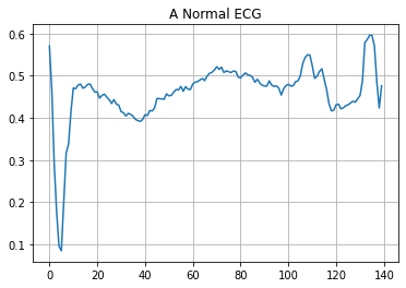
Plot an anomalous ECG.
plt.grid()
plt.plot(np.arange(140), anomalous_train_data[0])
plt.title("An Anomalous ECG")
plt.show()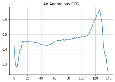
Build the model
class AnomalyDetector(Model):
  def __init__(self):
    super(AnomalyDetector, self).__init__()
    self.encoder = tf.keras.Sequential([
      layers.Dense(32, activation="relu"),
      layers.Dense(16, activation="relu"),
      layers.Dense(8, activation="relu")])

    self.decoder = tf.keras.Sequential([
      layers.Dense(16, activation="relu"),
      layers.Dense(32, activation="relu"),
      layers.Dense(140, activation="sigmoid")])

  def call(self, x):
    encoded = self.encoder(x)
    decoded = self.decoder(encoded)
    return decoded

autoencoder = AnomalyDetector()
autoencoder.compile(optimizer='adam', loss='mae')Notice that the autoencoder is trained using only the normal ECGs, but is evaluated using the full test set.
history = autoencoder.fit(normal_train_data, normal_train_data,
          epochs=20,
          batch_size=256,
          validation_batch_size=40,
          validation_data=(test_data, test_data),
          shuffle=True)
Epoch 1/20
10/10 [==============================] - 5s 176ms/step - loss: 0.0571 - val_loss: 0.0521
Epoch 2/20
10/10 [==============================] - 0s 16ms/step - loss: 0.0524 - val_loss: 0.0493
Epoch 3/20
10/10 [==============================] - 0s 15ms/step - loss: 0.0453 - val_loss: 0.0451
Epoch 4/20
10/10 [==============================] - 0s 15ms/step - loss: 0.0376 - val_loss: 0.0408
Epoch 5/20
10/10 [==============================] - 0s 15ms/step - loss: 0.0309 - val_loss: 0.0384
Epoch 6/20
10/10 [==============================] - 0s 14ms/step - loss: 0.0266 - val_loss: 0.0369
Epoch 7/20
10/10 [==============================] - 0s 15ms/step - loss: 0.0244 - val_loss: 0.0357
Epoch 8/20
10/10 [==============================] - 0s 17ms/step - loss: 0.0230 - val_loss: 0.0347
Epoch 9/20
10/10 [==============================] - 0s 15ms/step - loss: 0.0219 - val_loss: 0.0344
Epoch 10/20
10/10 [==============================] - 0s 15ms/step - loss: 0.0212 - val_loss: 0.0342
Epoch 11/20
10/10 [==============================] - 0s 14ms/step - loss: 0.0207 - val_loss: 0.0340
Epoch 12/20
10/10 [==============================] - 0s 16ms/step - loss: 0.0205 - val_loss: 0.0340
Epoch 13/20
10/10 [==============================] - 0s 15ms/step - loss: 0.0204 - val_loss: 0.0341
Epoch 14/20
10/10 [==============================] - 0s 15ms/step - loss: 0.0203 - val_loss: 0.0341
Epoch 15/20
10/10 [==============================] - 0s 15ms/step - loss: 0.0203 - val_loss: 0.0335
Epoch 16/20
10/10 [==============================] - 0s 15ms/step - loss: 0.0202 - val_loss: 0.0335
Epoch 17/20
10/10 [==============================] - 0s 14ms/step - loss: 0.0202 - val_loss: 0.0332
Epoch 18/20
10/10 [==============================] - 0s 15ms/step - loss: 0.0201 - val_loss: 0.0334
Epoch 19/20
10/10 [==============================] - 0s 16ms/step - loss: 0.0201 - val_loss: 0.0330
Epoch 20/20
10/10 [==============================] - 0s 14ms/step - loss: 0.0200 - val_loss: 0.0330plt.plot(history.history["loss"], label="Training Loss")
plt.plot(history.history["val_loss"], label="Validation Loss")
plt.legend()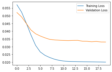
You will soon classify an ECG as anomalous if the reconstruction error is greater than one standard deviation from the normal training examples. First, let’s plot a normal ECG from the training set, the reconstruction after it’s encoded and decoded by the autoencoder, and the reconstruction error.
encoded_data = autoencoder.encoder(normal_test_data).numpy()
decoded_data = autoencoder.decoder(encoded_data).numpy()

plt.plot(normal_test_data[0], 'b')
plt.plot(decoded_data[0], 'r')
plt.fill_between(np.arange(140), decoded_data[0], normal_test_data[0], color='lightcoral')
plt.legend(labels=["Input", "Reconstruction", "Error"])
plt.show()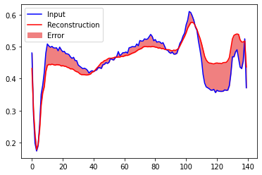
Create a similar plot, this time for an anomalous test example.
encoded_data = autoencoder.encoder(anomalous_test_data).numpy()
decoded_data = autoencoder.decoder(encoded_data).numpy()

plt.plot(anomalous_test_data[0], 'b')
plt.plot(decoded_data[0], 'r')
plt.fill_between(np.arange(140), decoded_data[0], anomalous_test_data[0], color='lightcoral')
plt.legend(labels=["Input", "Reconstruction", "Error"])
plt.show()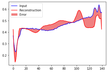
Detect anomalies
Detect anomalies by calculating whether the reconstruction loss is greater than a fixed threshold. In this tutorial, you will calculate the mean average error for normal examples from the training set, then classify future examples as anomalous if the reconstruction error is higher than one standard deviation from the training set.
Plot the reconstruction error on normal ECGs from the training set
reconstructions = autoencoder.predict(normal_train_data)
train_loss = tf.keras.losses.mae(reconstructions, normal_train_data)

plt.hist(train_loss[None,:], bins=50)
plt.xlabel("Train loss")
plt.ylabel("No of examples")
plt.show()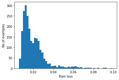
Choose a threshold value that is one standard deviations above the mean.
threshold = np.mean(train_loss) + np.std(train_loss)
print("Threshold: ", threshold)Threshold: 0.032062344Code language: CSS (css)Note: There are other strategies you could use to select a threshold value above which test examples should be classified as anomalous, the correct approach will depend on your dataset. You can learn more with the links at the end of this tutorial.
If you examine the reconstruction error for the anomalous examples in the test set, you’ll notice most have greater reconstruction error than the threshold. By varing the threshold, you can adjust the precision and recall of your classifier.
reconstructions = autoencoder.predict(anomalous_test_data)
test_loss = tf.keras.losses.mae(reconstructions, anomalous_test_data)

plt.hist(test_loss[None, :], bins=50)
plt.xlabel("Test loss")
plt.ylabel("No of examples")
plt.show()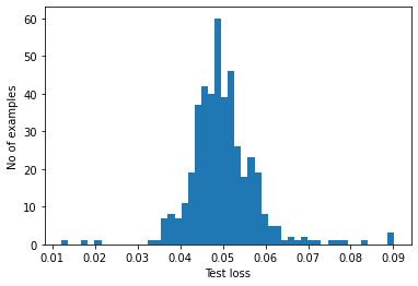
Classify an ECG as an anomaly if the reconstruction error is greater than the threshold.
def predict(model, data, threshold):
  reconstructions = model(data)
  loss = tf.keras.losses.mae(reconstructions, data)
  return tf.math.less(loss, threshold)

def print_stats(predictions, labels):
  print("Accuracy = {}".format(accuracy_score(labels, predictions)))
  print("Precision = {}".format(precision_score(labels, predictions)))
  print("Recall = {}".format(recall_score(labels, predictions)))
preds = predict(autoencoder, test_data, threshold)
print_stats(preds, test_labels)Accuracy = 0.943
Precision = 0.9941060903732809
Recall = 0.9035714285714286Copyright© 2021 Habana Labs, Ltd. an Intel Company.
Copyright 2020 The TensorFlow Authors.
Licensed under the Apache License, Version 2.0 (the “License”);
you may not use this file except in compliance with the License. You may obtain a copy of the License at https://www.apache.org/licenses/LICENSE-2.0 Unless required by applicable law or agreed to in writing, software distributed under the License is distributed on an “AS IS” BASIS, WITHOUT WARRANTIES OR CONDITIONS OF ANY KIND, either express or implied. See the License for the specific language governing permissions and limitations under the License.