Training Llama and Bloom 13 Billion Parameter LLMs with 3D Parallelism on Habana® Gaudi2®

This means either parallelizing the data or model or both to distribute computation across several devices.  Different forms of parallelism exist, and they can be combined to facilitate efficient training of LLMs. DeepSpeed [2] is a popular deep learning software library which facilitates compute- and memory-efficient training of large language models. Megatron-LM is a highly optimized and efficient library for training large language models using model parallelism [12]. DeepSpeed’s training engine provides hybrid data and pipeline parallelism, and this can be further combined with model parallelism such as Megatron-LM. Thus, data parallelism, Pipeline parallelism and tensor parallelism (horizontal model parallelism) can be combined to achieve 3D parallelism for training LLMs. These models can be trained on Habana Gaudi2 accelerators with Habana’s DeepSpeed fork, Megatron LM and Habana’s SynapseAI(R) software. In this article, we will talk about what 3D parallelism is and how it is useful for training LLMs. We will provide a brief overview of how one can train LLama 13B [10] and BLOOM 13B [11] LLMs using 3D parallelism on Habana Gaudi2. More details on DeepSpeed support on Habana SynapseAI Software can be found at Habana DeepSpeed User Guide. Now, let us dive into what are the different forms of parallelism and how we can use DeepSpeed, Megatron LM and Habana SynapseAI Software to train LLMs with these parallelism modes.

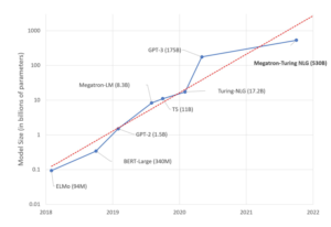
As the size of LLMs keeps growing, how can we efficiently train such large models?  Of course, the answer is “parallelization”. There are different parallelization techniques that can be applied to make the training compute and memory efficient. Parallelism can be obtained by splitting either the data or the model across multiple devices.

At a very high level, the two major types of parallelism are data parallelism and model parallelism. In Data Parallel training, each data parallel process/worker has a copy of the complete model, but the dataset is split into N_d parts where N_d is the number of data parallel processes. Say, if you have N_d devices, you split a mini batch into N_d parts, one for each of them. Then you feed the respective batch through the model on each device and obtain gradients for each split of the mini batch. You then collect all the gradients and update the parameters with the overall average. Once we get all the gradients (needs synchronization here), we calculate the average of the gradients, and use the average of the gradients to update the model/parameters. Then we move on to the next iteration of model training. The degree of data parallelism is the number of splits and is denoted by N_d.

Tensor Parallelism and Pipeline Parallelism

With model parallelism, instead of partitioning the data, we divide the model into N_m parts, typically where N_m is the number of devices. Model Parallelism requires considerable communication overhead. Hence it is effective inside a single node but may have scaling issues across nodes due to communication overhead.  Also, it is complex to implement. A large language model consists of multiple layers, with each layer operating on tensors. In model parallelism, we can choose to split the model within each layer with each model layer being split across multiple devices. This is the intra-layer model parallelism also known as tensor parallelism. In tensor parallelism, we shard the tensors across multiple devices so that each layer is computed in parallel across multiple devices.  

In contrast to tensor parallelism, we can choose to split a model at one or more model layer boundaries, as in the case of inter-layer model parallelism. This is also known as pipeline parallelism. Pipeline parallelism was first proposed in the GPipe paper [4]. Pipeline parallelism is intuitively very similar to the way normal factory assembly pipelines operate. In this case, a model is split into multiple stages (a stage can consist of one or more model layers) and each stage is assigned to a separate Gaudi device. The output of one stage is fed as input to the next stage. As a trivial example, let us consider a Multi Layer Perceptron (MLP) model with 4 layers and we will assign one layer each to each Gaudi device. However, this naïve splitting results in device under-utilization since only one device is active at a time, as shown in Figure below.

Figure 1 above [6] represents a model with 4 layers placed on 4 different devices (vertical axis). The horizontal axis represents training this model through time demonstrating that only 1 device is utilized at a time. To alleviate this problem, pipeline parallelism splits the input minibatch into multiple micro-batches and pipelines the execution of these micro-batches across multiple devices. This is outlined in the figure below:

Figure 2 above [6] represents a model with 4 layers placed on 4 different devices (vertical axis). The horizontal axis represents training this model through time demonstrating that the devices are utilized more efficiently. However, there still exists a bubble (as demonstrated in the figure) where certain devices are not utilized.  Pipeline parallelism while being simple to understand and implement can have these computation inefficiencies due to device under-utilization. Also, since the output of the previous stage needs to be fed to next stage, pipeline parallelism can result in communication overhead if this communication needs to happen across nodes rather than between devices on the same node.

While pipeline parallelism splits the model at the boundary of layers, tensor parallelism splits the model intra-layer by sharding the tensors at each layer. Tensor parallelism was described in the Megatron [3] paper and is quite complex to implement. However, it is more efficient than pipeline parallelism. As a trivial example, let us consider a 2 layers MLP model with the parameters of layer 1 represented by matrix A and layer 2 represented by matrix B respectively with input data batch being X and output of MLP being Z.  Typically, we would need to compute  Y = f(XA) where f is the activation function and the output of MLP would be Z = YB.   With tensor parallelism, we can split both the matrices into 2 pieces and place them on two devices as shown below in Figure 3, where matrix A is split into two equal parts column-wise, and matrix B is split into two equal parts row-wise.

We can rewrite the above computation using the sharded tensors as below:

Yi ​  = f (XAi​)   for i∈{1,2}
Zi ​= YiBi ​for i∈{1,2}
Z = Z1 ​+ Z2​ 

While the above equations describe the forward pass with tensor parallelism, backward pass equations can also be rewritten to use the sharded tensors. A detailed description of pipeline parallelism and tensor parallelism can be found in [6].

What is 3D Parallelism?

As discussed above, we have three kinds of parallelism namely data parallelism, tensor parallelism (often referred to simply as intra-layer model parallelism) and pipeline parallelism (often referred to as inter-layer model parallelism).  DeepSpeed and Megatron LM are libraries that enable efficient training of LLMs by the following:  

• Memory efficiency: Model is split using pipeline parallelism first and then further each pipelined stage is split using tensor parallelism. This 2D combination simultaneously reduces the memory consumed by the model, optimizer, and activations. However extreme partitioning can lead to communication overhead which will impact compute efficiency.
• Compute efficiency: To scale beyond tensor and pipeline parallel approaches, data parallelism is leveraged [1]
• Topology aware 3D mapping: The three forms of parallelism are carefully combined to optimize for intra-node and inter-node communication overheads.

A detailed description of 3D parallelism can be found in [6,7,8]. The following figure demonstrates how 3D parallelism can be leveraged using  DeepSpeed and Megatron LM techniques  This example shows how 32 workers are mapped across 8 nodes with each node hosting 4 Gaudi devices. Layers of the neural network are divided among four pipeline stages. Layers within each pipeline stage are further partitioned among four model parallel workers. Lastly, each pipeline is replicated across two data parallel instances.

Training Llama-13B on Habana Gaudi-2 with 3D Parallelism

Now that we have understood the 3D parallelism mechanism, let us briefly turn our attention to how we can train an LLM using this feature. We use LLama-13B as the example LLM.  Llama is a family of Large Language Models  based on transformer architecture and trained on over one trillion tokens with various enhancements such as Rotary Position Embeddings, SwiGLU activation function, Pre-normalization and use of AdamW optimizer. Full technical specifications of the Llama Model can be found in [10].

We trained a LLama-13B model using Habana SynapseAI(R) Software version 1.10.0 with Pytorch 2.0.1, DeepSpeed 0.7.7 software library, with our training implementation based on https://github.com/microsoft/Megatron-DeepSpeed. Detailed steps for training Llama-13B and large models of similar sizes can be found here. The command for training is given below:

HL_HOSTSFILE=scripts/hostsfile HL_NUM_NODES=8 HL_PP=2 HL_TP=4 HL_DP=8 scripts/run_llama13b.sh

HL_NUM_NODES specifies the number of nodes involved in the run, HL_PP is used to set up the pipeline parallelism factor and HL_TP variable is used to set the tensor parallelism factor and HL_DP is the data parallelism factor.  HL_HOSTSFILE contains the IP addresses of the respective HPU nodes.  The run script for training sets up the important variables as shown below:

NUM_NODES=${HL_NUM_NODES}

DP=${HL_DP}

TP=${HL_TP}

PP=${HL_PP}

With 64 Gaudi2 devices, and with BF16 precision, we were able to achieve 55.48 sentences per second throughput in training the Llama-13B model with SynapseAI 1.11.

Training Bloom-13B on Habana Gaudi-2 with 3D Parallelism

While we discussed 3D parallelism enabled training for training LLama 13B model, we can use the same setup to train other large models including Bloom-13B [11] model as shown here,

For multicard configurations, for example to run Bloom on 32 Gaudi2 devices with BF16 precision, the run command would be as given below with HL_HOSTSFILE containing the IP addresses of the respective HPU nodes.

HL_HOSTSFILE=scripts/hostsfile HL_NUM_NODES=4 HL_PP=2 HL_TP=4 HL_DP=4 scripts/run_bloom13b.sh

For running training with 64 devices, we modify this command by changing HL_NUM_NODES and HL_DP as shown below:

HL_HOSTSFILE=scripts/hostsfile HL_NUM_NODES=8 HL_PP=2 HL_TP=4 HL_DP=8 scripts/run_bloom13b.sh

With 128 devices and with BF16 precision, the throughput was 114.1 samples/sec. This corresponds to 15.6 days for the completion of the training run to achieve convergence. The figure below shows the training loss (lm-loss) plotted against the number of training iterations. The blue colored curve is the training loss measured on HPU (with bf16) whereas the orange colored curve is the training loss from the BigScience Bloom Reference implementation [11] which used FP16.

If you want to train a large model using Megatron-DeepSpeed, but the model you want is not included in the implementation, you can port it to the Megatron-DeepSpeed framework. For details on porting your own model to Megatron-DeepSpeed framework, please refer to this document.

Get started on your Generative AI journey on the Habana Gaudi2 platform today. If you would like to get access to Gaudi2 for your LLM training needs, sign up on the Intel Developer Cloud following the instructions here or contact Supermicro regarding Gaudi2 Server infrastructure.

Happy & Speedy Model Training with Habana Gaudi2, SynapseAI and DeepSpeed!

References

1. DeepSpeed: Extreme-scale model training for everyone
2. Pytorch blog on pipeline parallelism
3. Megatron LM paper
4. Gpipe paper.
5. PipeDream paper
6. Tensor parallelism vs pipeline parallelism
7. https://huggingface.co/docs/transformers/v4.15.0/parallelism
8. Deepspeed tutorial on pipeline parallelism
9.  What Language Model to Train if You Have One Million GPU Hours?
10. LLaMA: Open and Efficient Foundation Language Models
11. BLOOM: A 176B-Parameter Open-Access Multilingual Language Model
12. https://github.com/NVIDIA/Megatron-LM